ArcPad Data Collection

Introduction
Throughout my college career, I have used various GPS devices for navigation and data collection.  However, I had previously never created a geodatabase to be deployed in the field to be used for data collection.  This report will summarize the process of developing a data collection procedure from the ground up.  This process begins with creating a geodatabase and feature classes.  Domains will be set for the feature classes to aid in the data collection process in the field.  Finally, the geodatabase will be saved to a Trimble Juno GPS unit for data collection.

Figure 1. Trimble Juno to be used to collect GPS data

Study Area
This weeks assignment consisting of ArcPad data collection took place at the Priory.  This land, purchased by the university to be a day care facility, is located to the south of the city of Eau Claire. Figure 2 shows the mostly wooded areas surrounding the building that we have previously used for navigation exercises. 

Figure 2. Study Area

Methods
My group began this assignment by considering the terrain and features at the priory that we could collect multiple attributes for.  We decided to mark the locations we found garbage and signs at the priory.  The next step was to build a geodatabase containing the features and attributes that would be collected.  A new geodatabase was created, as well as "Garbage" and "Signs" feature classes.  The Garbage feature class contained garbage material, garbage size, garbage type, and notes fields, and the Signs feature class had sign color, sign material, sign type, and notes.  To aid in the data collection process, domains were created to allow us to simply select a predetermined option rather than having to type in each attribute.  Once the feature classes were created and the domains were set, their symbology was changed so that they could be differentiated on the Juno when we were out in the field.  The features and an aerial image were added to a blank ArcMap document, and then saved to the Juno using the ArcPad Data Manager toolbar.
           
Once the was saved on the Juno, we were able to go out in the field and begin to collect data using ArcPad.  My group began in the parking lot marking the locations of signs and garbage as it was found.  We then moved to the north and followed a trail where trail marker signs were mapped.  Figure 3 shows the route the we took, as well as the locations of all signs and garbage.

Figure 3. Locations of Signs and Garbage at the Priory

After the data collection, the data was extracted from the Juno by simply copying and pasting the folder back into the Priory folder that I had previously created on the computer.  I examined the data, and then created a series of maps to symbolize the different attributes that we collected. 

Discussion
Having already created the domains for each feature, the data collection was seamless and went very well.  We were able to select from a preset list of options for each attribute which allowed the collection to be very quick and efficient.  The only exception was when the garbage or sign had an attribute that was not part of the domain.  When this occurred, the "other" option was selected and the attributed was specified in the notes field.  Figures 4, 5, and 6 display the garbage material, type, and size of items that were found at the priory.  Most of the garbage items found were plastic bottles, aluminum cans, and plastic bags.  These items were all found near the parking lot for the priory, which makes sense because it is the area where people are the most.

Figure 4. Garbage Material

Figure 5. Garbage Types



Figure 6. Garbage Size

Figures 7, 8, and 9 contain maps symbolizing the attributes collected about signs.  There were many informational signs surrounding the parking lot about parking information.  At the southern extent of the maps, there are dots representing a stop sign on the left, and the priory sign on the right.  The orange signs marking the trail can be seen to the north of the priory building. 

Figure 7. Sign Type

Figure 8. Sign Color

Figure 9. Sign Material

ConclusionThis assignment proved to be a great introduction to the preparation of gathering data in the field.  A geodatabase was first created, along with the two feature classes that our group decided to map (Signs and Garbage).  Domains were then set to provide us with attribute options in the field.  This was very helpful and speeded up the process because we could quickly select an option, rather than having to type in the word.  After the domains were set, the data was saved onto a Trimble Juno GPS unit.  ArcPad was utilized to collect the garbage and signs data at the priory, and following the field work, the data was dowloaded and a series of maps were created to symbolize the different attributes.

HABL Launch

Introduction
Over the course of the semester, our class has spent a lot of time using balloons to collect aerial imagery of our campus.  In addition to those mapping activities, we also created a rig for what we called the HABL (High Altitude Balloon Launch).  This activity involved launchig a balloon into space while recording video of the flight.  The balloon was to travel about 100,000 feet up until it popped due to the pressure.  The parachute would then open up and bring the camera rig back down to surface.    


Methods
The construction of the HABL rig began a few months ago, with design modifications occurring after some of the other balloon mapping exercises.  Figure 1 shows the container used to house the camera for this activity made out of a styrofoam bait container.  A hole was cut out of the bottom for the camera lense to take video during its flight.  The rig also contained a water proof case for the camera, handwarmers to keep the camera from getting too cold, and a tracking device to that we could recover the rig after it came back down to the surface.  Four strings were connected from the edges of the rig and tied together at the top.

Figure 1. Rig designed to house the video camera for HABL launch

Figure 2 shows the balloon being walked to the balloon launching site in the middle of the campus mall.  The balloon was filled from a large helium tank until it was about eight feet in diameter.  We did not want to fill the balloon up too much because the balloon needs to expand as it gets to higher altitudes.  After the balloon was filled to the desired amount, zip ties and duct tape were used to seal off the balloon.  The rig containing the camera and parachute were then attached using carabiners.  After watching the weather closely for a few weeks, the launch was finally scheduled for 10 AM on April 26. 

Figure 2. Balloon being walked to the launch site

Here is a link to a video that was taken of the launch. 
http://desi.uwec.edu/Geography/Hupyjp/Weather_Balloon_1024.asx
As soon as the balloon was let go, winds immediately took it to the east.  The tracking device stopped working (most likely from cool temperatures), but fortunatly about an hour and a half later we got a stationary signal indicating that the balloon had touched down.  Our professor and a few students set out to retrieve the balloon rig which touched down near Marshfield, WI.  Upon arrival, they found the rig stuck in a tree (Figure 3).  Our professor climbing up the tree and cut one of the limbs off to retrieve the rig.       

Figure 3. HABL rig stuck up in a tree

Discussion
The HABL turned out to be a success, as we were able to collect some great video of its journey.  In the course of an hour and a half, the balloon traveled about 100,000 feet up in the air and about 78 miles to the southeast.  Figure 4 shows the distance traveled by the balloon rig. 


Figure 4. Distance traveled by balloon rig

Figures 5, 6, and 7 show some images extracted from the video footage. 


Figure 5. Still shot from the camera of the campus footbridge

Figure 6. Still shot of the Chippewa River to the east of Eau Claire

Figure 7. Image at the peak of the HABL launch where the curvature of the Earth is visible

Although our main goal of recovering the camera was fulfilled, there were some aspects of this activity that could have been improved.  Condensation covered the lens of the camera at higher altitudes and left some of the footage to be a bit hazy.  As previously mentioned, the tracking device stopped working during the flight but did function properly after it landed.  It would have been cool to watch the flight in real time.  Also, the camera that was used only had a capacity to take video for one hour so the full descent of the balloon was not captured.   

Conclusion
This activity was really a culmination of efforts throughout the entire semester and was based on trial and error.  Balloon mapping is not very widespread, so there was not much information about it, leaving us to work together make this activity work.  I feel very fortunate to have been able to have been a part of something as an undergrauate student that not many people have a chance to participate in.  Overall, I thought the aerial image gathering and HABL using balloons were some of the coolest projects I have been a part of in college.  In the future, this class plans to include a GPS unit, thermometer, barometer, and anemometer to be able to gather more data during the flight.         

Balloon Mapping Final Report

Introduction
Our geospatial fields methods class has been thinking conceptually about and working on an aerial mapping project of the University of Wisconsin - Eau Claire campus for a while.  Early on in the semester we did extensive research on the topic, and found that there was not a lot of information about it on the internet.  Therefore, we have been almost "winging it" and coming up with ideas on the procedure by ourselves.  Now that the weather has warmed up a little bit, we were able to finally put the project into action.

Methodology
Day 1:
We previously had constructed contraptions out of two-liter soda bottles to hold the camera in for the project, but those ideas have since been scrapped.  A small styrofoam container is now being used to house the camera for the project.  A hole was cut out of the bottom of the container for the camera to take pictures through.  The first task of the day was to inflate the balloon.  This was done by attaching a hose from a helium tank and inserting it into the opening of the balloon (Figure 1).

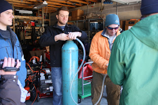
Figure 1. Helium tank/hose

Figure 2 shows the balloon as it was being inflated with helium.  The balloon was inflated until it had a diameter of about five and a half feet wide.

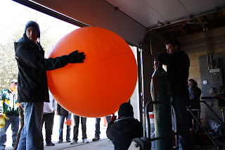
Figure 2. Inflating the balloon

After the balloon was inflated, zip ties were used to clamp the opening shut around a rubber ring.  Then, a carabiner was put on to the ring to attach it to the string that we would use to hold on to the balloon.  The string was measured and marked into 100 foot increments.  It was determined that the balloon was going to be let out 400 feet.  The styrofoam contraption housing the camera and a Garmin eTrex GPS unit were also attached (Figure 3).  

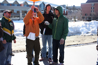
Figure 3. Attaching the camera contraption to the balloon

Continuous shot mode was turned on on the camera, and the shutter button was fastened down to continuously take pictures using rubber bands and tape.  Once everything was attached to the balloon, 400 feet of string was let out and the balloon mapping began.

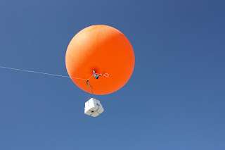
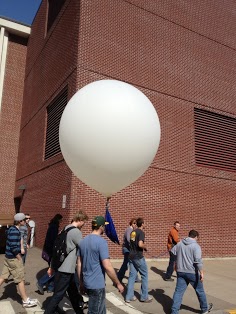
Figure 4. Balloon being let out on the string

The class then began walking around campus, using care to guide the balloon through areas without getting the line snagged on trees or power lines.  This video shows the conclusion of the exercise.  We were just beginning to wind the string back in and bring the balloon down when something broke on the line due to severe tension caused by the heavy winds that were blowing on this day.  The balloon floated away and the container that had the camera inside of it fell into the river that flows through campus.  We were, however, able to retrieve the camera and get the pictures that were taken.    

The images that were taken were then to be mosaicked together to create one large aerial image of campus.   One method of mosaicking that I had no previous experience with and wanted to try was using http://mapknitter.org/.  This is a very user-friendly website for mosaicking.  The site provides aerial imagery, and the user simply loads images on top of that imagery.  The images are then dragged to their correct location, and can be resized, rotated, and distorted to combine the images together.
The map that I made using this site can be found here: http://mapknitter.org/map/view/uweccampus.

Day 2:
We decided to construct a different system for housing the camera for the second class of balloon mapping.  The winds during the previous class kept swinging the styrofoam container around, causing many images to be taken at oblique angles.  In order to make the more aerodynamic, the camera was attached to an arrow (Figure 5).  This would allow the wind to flow around the device, and hopefully reduce the amount of swinging around from side to side up in the air.

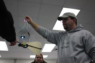
Figure 5. New device to hold the camera

The following videos document the process of inflating the balloon and attaching the camera to the string on the balloon.  This time, a metal ring instead of a rubber one was used to secure the various parts together.  

We were able to walk the balloon around and obtain imagery covering almost the entire campus.  The images were georeferenced and mosaicked together using ArcMap.  In order to save time, the campus was divided into six different sections.  Groups were then assigned to an area and were in charge of georeferencing images for that area.  Each group was then supposed to import a mosaic of their area into a geodatabase for a final mosaic of the entire campus.

Georeferencing is a relatively straight-forward process in ArcMap.  The first step is to obtain a reference image for the desired area.  The images that you want to georeference are then added to the document.  It is best to find images that are taken looking straight down towards the ground to limit the amount of distortion.  Enough images should be selected so that there is about a 60% overlap in the area covered by the image.  The georeferencing toolbar is then turned on and used to select the image that you want to georeference.  Using the add control points button, a point on the image is clicked, followed by clicking on the corresponding spot on the reference image.  Each image should have at least nine control points added to it to ensure an accurate georeference.   Figure 6 shows an image being georeferenced with its control points displayed.

Figure 6. Image with control points

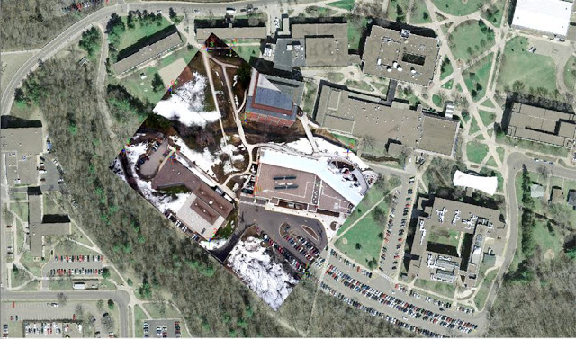
Once all of the control points are added and the image is georeferenced properly, the image must be rectified.  This updates the georeferencing and saves the image as a new file.  Then, the next image is selected and the process is repeated until all of the images are georeferenced.  When all of the georefencing is done, the Mosaic to New Raster tool was used to mosaic the images together.  Figure 7 shows the final mosaic of the area that my group was assigned.

Figure 7. Mosaic

One issue that arose during the geoferencing process was the string being visible in some of the images.  I tried choosing images where the overlap would remove the string, but it is still visible in two of the images in the mosaic.

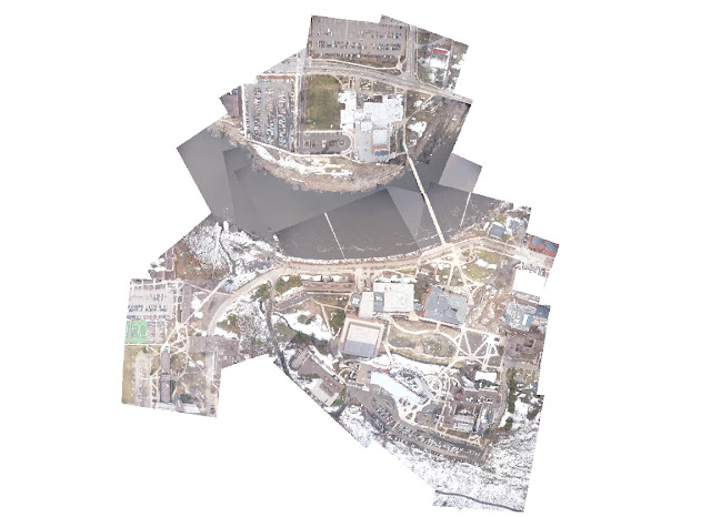
Figure 8. Mosaic of Entire Campus

Discussion
We were able to take away quite a bit of knowledge from the first day of balloon mapping.  It was a very windy day, which influenced the quality of images we got, and ultimately led to the loss of the balloon.  Therefore, the weather conditions must be considered for a project like this.  A sunny day with calm or gentle winds would be ideal.  When the balloon was up in the air, the wind tossed around the styrofoam box that contained the camera.  This led to the camera taking many pictures at odd angles.  Those images were distorted, and not useful at all for creating a mosaic.  Because of that issue, we decided to create a new contraption for housing the camera for the second day of balloon mapping utilizing an arrow.  This was much more aerodynamic, and we were able to get better pictures facing straight down.  The high winds also affected the flight of the balloon.  Rather than rising straight up, the balloon was pushed way off to the side (Figure 4).  This severely shortened the elevation of the balloon up in the air and limited the expanse of coverage of the images taken by the camera.    

Due to recent construction on campus, there are no reference images that are up to date.  This made the georeferencing of some areas very difficult.  A few members of the class attempted to take ground control points using various GPS units.  There was a discrepancy in the location of points among the various units so I chose not to use the points during the georeferencing process.

Conclusion
The two balloon mapping sessions turned out to be very successful, despite losing the balloon on the first launch.  We were able to get many good images of campus to georeference and mosaic together.  The first class of balloon mapping also provided us with a lot of information to make the second attempt much better.  We learned what effect the weather could have on a project like this, and created a better device to hold the camera for the second launch.  In addition to using ArcMap to georeference and mosaic the images, I was also introduced to Map Knitter, which is a website where you can add images together on top of an aerial image.

Balloon Mapping

Introduction
Our class is embarking on an aerial mapping project of our college campus.  A large helium balloon was used with a camera attached facing downwards.  A long string was then tied to the balloon so we could move the balloon around campus, as well as set the desired altitude of the balloon.     

Methodology
The imagery was gethered using a large balloon that was launched into the air about 400 feet.  Attached to the balloon was a camera facing downwards.  Once the balloon was at the desired altitude, we walked all around campus to collect as much imagery as possible.  After this process was completed, the images from the camera were located onto the computer.  Relevant images pertaining to the assigned area were selected and were georeferenced.  Georeferencing is accomplished by adding control points to the image and matching them to the corresponding location on another image that is already georeferenced.  The first step in this process is to display an already georeferenced image, followed by turning the georeferencing toolbar on.  An image that needs to be georeferenced is then loaded, and fit to the display. 

Figure 1. Aerial image to be georefenced displayed.

Using the add control points tool, a control point is clicked on the image, and then again on the corresponding location on the already georeferenced image.  These control points can consist of the corners of buildings or sidewalks, trees, or any other distinctive featuers.  This process is repeated until the image appears to be in the correct location.  When georeferencing my images, I tried to have at least 10 points.

Figure 2. Aerial image with control points displayed.

Once done georeferencing an image, it must be rectified to be saved as a new file.  Then, other images are added to the display and georeferenced until the desired area is covered by the newly georeferenced images.

Figure 3. Additional images being added and georeferenced.

When all of the desired images are georeferenced, the mosaic to new raster tool is employed to combine the images into one file.

Conclusion
Figure 4 shows the final mosaic of the images that I georeferenced. 


Figure 4. Final mosaic of imagery.

Final Navigation Report

Introduction
Over the past few weeks, our Geospatial Fields Methods class has been participating in different land navigation techniques.  This process began by spending the first week establishing pace counts for each person in the class and creating maps that would be used for navigation with a compass.  The next week, we were put into groups and assigned six points that we were to navigate to using traditional map and compass navigation.  The next field outing consisted of navigation to a different set of six points using just a Garmin eTrex GPS unit.  The field outings concluded this past week with a final navigation activity that incorporated paintballing.  Each group was to navigate to as many points possible with the use of a GPS unit and maps that were created.

Study Area
Our field navigation exercises took place on the lands surrounding The Priory, which is located just to the south of the city of Eau Claire.  An aerial image of the area, navigation points, and 5-meter contours can be seen in Map 1.  

Map 1. Study Area

The aerial image shows that the study area is mostly wooded with a few distinct features that aided in the navigation.  These included the highway and waste pond bordering the area to the north, the planted pine tree region to the east, and the ridge stretching through the area as evidenced by the contours.  

Methodology
Week 1
In preparation for the first week's field outing, we needed to establish our pace count and create the navigation maps that we were to use out in the field.  Our pace count was established by marking off a distance of 100 meters and counting the number of paces it took us to walk it.  I found my pace count to be 65.  To create the navigation maps, data such as a orthophotograph, two-foot contour lines, five-foot contour lines, and a DEM was used.  A UTM grid was also placed over the map to aid in the navigation.  Each group member created two maps for the event and then as a group, two final maps were selected to use in the exercise (Maps 2 and 3).

Map 2. My map for traditional land navigation exercise.

Map 3. Hannah's map for traditional land navigation exercise

Week 2
On the day of the field event, we plotted the locations of the points that our group was assigned to navigate to.  Straight lines were then drawn from point to point, and a compass was used to measure the bearing.  

Figure 1. Mitch and Hannah plotting points. 

We then went out in the field and began our navigation event.  Our group utilized a three-person system for the exercise.  One person had the compass and would direct a person to walk to a specified location on the bearing.  The final person would then walk to that person and count the number of paces to estimate the distance traveled.  This process was repeated until our navigation points were located. 

Figure 2. Mitch standing at point marker and directing Hannah towards next location.

Week 3
The next week, we were to use GPS units to navigate to the points rather than using the traditional land navigation techniques using a map and compass.  Each student was assigned a Garmin eTrex GPS unit for the activity.  The unit would be used to locate the navigation points that we were assigned and to track the routes that were taken while navigating to the points.  My group was assigned the points on Course 3, with point 1B being our starting point and heading to the other points in order.  

Table 1. Navigation Points

My group utilized the UTM coordinates to navigate to the points.  To get to the points, we generally began by navigating to the correct x value, and then walked to arrive at the correct y value.  A recent snowstorm made walking slow and a bit difficult.

Figure 3.  Hannah and I examining our GPS units at a point marker.

After we navigated to all of the points, we returned to the parking lot where the class was congregating and turned off the tracking on the GPS units.  This data was then uploaded as a shapefile using the Minnesota DNR Garmin Application.  The shapefile was uploaded in the NAD 1983 UTM Zone 15N projection to be consistent with the other files that were used for mapping of the priory area.  Each student's track log was then imported into a feature dataset which allowed for access of all of the files for everyone.  This data was then used to create maps displaying the track log from my GPS unit, the track logs for my group, and a map containing the track logs of everyone in the class.

Week 4
The final activity incorporated paintballing into the navigation exercise.  Each group was to navigate to as many of the 18 navigation points as possible using a Garmin eTrex GPS unit and maps that we created for the event (Maps 5 and 6).  

Map 5. Paintball navigation exercise map. 

Map 6. Paintball navigation exercise map.

The maps were to aid the GPS units in the navigation to compare the ease of navigation to the previous week in which we only had GPS units.  The track logs were again turned on to track the locations of each person, and waypoints were to be taken at each of the point markers.  The rules for the paintball aspect was that if a person was shot, their group had to sit still for two minutes and not shoot at anyone.  We were also given the option of wearing snow shoes because of the high depth of snow still on the ground.  The activity began with a few minutes of non-shooting time while each of the six groups spread out to where they wanted to begin.  After the exercise, the waypoints and track logs were imported using the Minnesota DNR Garmin Application, and maps displaying my track log, my other group member's track log, and the track logs for everyone in the class were created.
  
Discussion
Overall, the different navigation events went very well for our group.  In the first activity using a map and compass, we were able to utilize a method that allowed us to move to the points quickly and efficiently.  However, there were a couple minor issues that we had to overcome.  The pace count that we established was done in a flat parking lot, and was not very conducive to estimating accurate distances when walking through the woods.  There were many hills that we had to walk up and down, as well as many trees and other obstacles that made walking in a straight line difficult.  When walking between points four and five, we came across some ponds that were fenced off.  In order to accurately maneuver around them, we counted a number of paces to the side of them.  Once we were around the ponds, those same number of paces were walked sideways to get back on the correct bearing. As mentioned earlier, we also the grid issue on Hannah's map that did not allow us to plot the UTM points.  Experiencing this shortcoming has stressed the importance of reviewing every detail before going out in the field.   

The maps that we prepared were great resources in the field.  The aerial imagery was very helpful in determining what type of terrain we were in and should be going to.  The DEM symbology and contours were also useful for tracking our progress on the map.  We had to walk up and down a few hills, and this information allowed us to make an accurate estimate of our location in terms of the points we were navigating to.  The point data we were given had the elevation in meters listed, and Map 2 that I created was useful because the five-foot contours were labeled.  For future navigation exercises, I would create maps very similar to the ones that we created for this event because the information we included on them was very helpful in the field.  One change would be to include the grid on both maps.  

After the completion of the second field outing, it was apparent that navigation with a GPS is easier and faster than traditional navigation with a map and compass.  GPS navigation does not require any preparation time, and it is much quicker in the field because a person can continuously walk and not have to worry about walking to a certain spot on the bearing and count the number of paces.  It also can be accomplished easily by oneself, whereas in the traditional method, a three person group is ideal.  Another advantage of GPS navigation is that a waypoint can be created on the GPS and it will tell you which direction and how far to travel to this location.  We did not do this during our navigation exercise, but this would have been very helpful and effective to do.   

Even with these benefits of GPS navigation, we did run into a few minor issues in the field.  It was very easy to misread some numbers when walking and looking at the GPS which led us a little out of our way a couple times.  An example of this can be seen in the animation of my track (http://www.youtube.com/watch?v=iP7FNiIi3xk) between points 3, 4, and 5.  When using UTM coordinates, it is important to remember that the x values increase as you move to the east, and y values increase as you move to the north.  A map accompanying the GPS unit can be very helpful to visualize this when determining the direction to travel.  This led us to the final navigation exercise where we had a map to accompany the GPS.  This method proved to the the quickest and most efficient method of land navigation.  Maps 7-12 display the track log data from each of the two navigation exercises where GPS units were used.  

Map 7. My track log from GPS navigation exercise.

Map 8. My track log from GPS and map navigation exercise. A green to red color ramp was used to symbolize the time.

Map 9. My group's track logs from GPS navigation exercise.

Map 10. My group's track logs from GPS and map navigation exercise.

Map 11. Class track logs from GPS navigation exercise.  I was assigned to Group 3.

Map 12. Class track logs from GPS and map navigation exercise.  I was assigned to Group 3.

When comparing the tracks from these two exercises, it is evident that the tracks taken between points are much more direct in the second exercise when we were allowed to have a map.  This is also apparent when the time data from the track logs is examined.  In the first GPS exercise, my group traveled to five points (not counting the starting point) in 1 hour and 18 minutes.  In contrast, my group traveled to 14 points in 2 hours and 28 minutes during the second exercise.  This also includes time that was spent engaging in fire with other groups.  The map was a great reference to use during the navigation, and eliminated time spent walking in the wrong, or not always most direct line to a point as seen in Map 7.  We were able to use the map to determine an efficient route in terms of the order the points would be navigated to.  Physical features such as the type of land cover and ridges that were evident from the map were also great references for the location of each point.  One trick that our group did not take advantage of, and would have helped immensely, was to use the coordinates of the navigation points and create waypoints in our GPS unit.  The GPS would then be able to give us the direction and distance we needed to travel to that point.  

Conclusion
These field navigation exercises provided an excellent understanding of three different navigation methods: traditional navigation with a map and compass, GPS navigation, and GPS navigation with the aid of a map.  My group was able to successfully navigate to points using these methods, and upon reflecting on them, decide which method was the easiest and most efficient.  This turned out to be navigation with a GPS and map.  Navigation with just a GPS unit is not a bad option, but having a map available all the time is not very conceivable.  Finally, the method of navigation with a map and compass was the slowest, but is still an effective option in cases where GPS technology is failing the user.

GPS Navigation

Introduction
Over the past few weeks, our Geospatial Fields Methods class has been exploring different land navigation techniques at The Priory.  First, the traditional technique of using a map and compass was used to navigate to six different point markers in a wooded area.  This week a Garmin eTrex GPS unit was used to navigate to six different points.  The GPS units had the tracking feature on, which was used to create maps and an animation showing the routes of students through the woods.  Next week we will be participating in a paintball activity that involves navigating to as many points as possible.  

Methodology
In preparation for last week's field outing, we needed to establish our pace count and create the navigation maps that we were to use out in the field.  Our pace count was established by marking off a distance of 100 meters and counting the number of paces it took us to walk it.  I found my pace count to be 65.  To create the navigation maps, data such as a orthophotograph, two-foot contour lines, five-foot contour lines, and a DEM was used.  A UTM grid was also placed over the map to aid in the navigation.  On the day of the field event, we plotted the locations of the points that our group was assigned to navigate to.  Straight lines were then drawn from point to point, and a compass was used to measure the bearing.  We then went out in the field and began our navigation event.  Our group utilized a three-person system for the exercise.  One person had the compass and would direct a person to walk to a specified location on the bearing.  The final person would then walk to that person and count the number of paces to estimate the distance traveled.    

This week, we were to use GPS units to navigate to the points rather than using the traditional land navigation techniques using a map and compass.  Each student was assigned a Garmin eTrex GPS unit for the activity.  The unit would be used to locate the navigation points that we were assigned and to track the routes that were taken while navigating to the points.  My group was assigned the points on course 3, and started at point 1B and then went to point 2B.  The other group that was assigned to course 3 started at point 1B and went to point 6B.

Table 1. Navigation Points

My group utilized the UTM coordinates to navigate to the points.  To get to the points, we generally began by navigating to the correct x value, and then walked to arrive at the correct y value.  A recent snowstorm made walking slow and a bit difficult.

Figure 1. Hannah and I examining our GPS units at a point marker.

After we navigated to all of the points, we returned to the parking lot where the class was congregating and turned off the tracking on the GPS units.  This data was then uploaded as a shapefile using the Minnesota DNR Garmin Application.  The shapefile was uploaded in the NAD 1983 UTM Zone 15N projection to be consistent with the other files that were used for mapping of the priory area.  Each student's track log was then imported into a feature dataset which allowed for access of all of the files for everyone.  This data was then used to create maps displaying the track log from my GPS unit, the track logs for my group, and a map containing the track logs of everyone in the class.

Map 1. Track log from my GPS unit.

This map shows the route that I took during the field navigation event.  Symbology was used to display the beginning of the track in a lighter color.  The color then gradually becomes darker as the track progresses.  This data was then used to create an animation of the track.  To do so, the file was selected as a time track under the properties.  The animation toolbar was then used to create and export the video.  The video can be found here: http://www.youtube.com/watch?v=iP7FNiIi3xk.  The files from the rest of the students in the class were added into ArcMap and maps were created to show their track logs.

Map 2. Group GPS Navigation Map

This map displays the track logs for Hannah and me.  Mitch's file was not in the file when it was accessed.  As you can see, Hannah's track log had much fewer points, and is most likely due to a difference in the increments that the GPS unit took points.  

Map 3. Class track logs.

Discussion

After the completion of this field outing, it was apparent that navigation with a GPS is easier and faster than traditional navigation with a map and compass.  GPS navigation does not require any preparation time, and it is much quicker in the field because a person can continuously walk and not have to worry about walking to a certain spot on the bearing and count the number of paces.  It also can be accomplished easily by oneself, whereas in the traditional method, a three person group is ideal.  Another advantage of GPS navigation is that a waypoint can be created on the GPS and it will tell you which direction and how far to travel to this location.  We did not do this during our navigation exercise, but this would have been very helpful and effective to do.   

Even with this benefits of GPS navigation, we did run into a few minor issues in the field.  It was very easy to misread some numbers when walking and looking at the GPS which led us a little out of our way a couple times.  An example of this can be seen in the video of my track between points 3, 4, and 5.  When using UTM coordinates, it is important to remember that the x values increase as you move to the east, and y values increase as you move to the north.  A map accompanying the GPS unit can be very helpful to visualize this when determining the direction to travel.  Finally, GPS technology can not always be relied upon so it is important to have an understanding of traditional navigation techniques.  The batteries in the unit could die, or you could be in an area where it is difficult to obtain a reliable signal.      

Navigation with a Map and Compass

Introduction
The objective for this week's exercise was to navigate through the woods to a series of points using a map and a compass.  This exercise is the follow-up activity to last week's prep work, consisting of the creation of maps and the establishment of each person's pace count.  

Methodology
The preparations for this week's field activity took place last week with the establishment of a pace count and creation of maps of the area of interest.  To establish each student's pace count, 100 meters was marked off in a parking lot.  We then walked the distance and counted the number of paces it took.  I walked the distance three times, and had a consensus pace count of 65.  Maps were then created of the area of land around the Priory using a variety of data sets (Maps 1 and 2).

Map 1. Priory Navigation Map with DEM and Two-Foot Contours

Map 2. Priory Navigation Map with Orthophoto and FiveMeter Contours

As a group, we chose to use Hannah's map in our navigation exercise (Map 3), as well as Map 2.

Map 3. Hannah's Navigation Map

 The field event took place the following week on March 4th.  A snowstorm was moving into the area, but there were only a few flurries during the exercise.  As previously mentioned, our goal was to navigate to five different points using a compass and the maps that we had created.  The first step in the process was to plot the points on our maps using the UTM coordinates that were given to us.  In attempting to do so, it was evident that the grid that Hannah put on her map was not correct.  This put our group in a quandary because there was no way for us to plot the points.  Luckily, we were able to use another group's map.  After the points were plotted on the new map that was given to us, a straight edge was used to draw lines connecting each of the points.  These lines were used to calculate the bearing.  To do so, the compass was placed on top of the map facing the direction that we wanted to travel.  The dial on the compass was then turned so the lines were facing straight up to the top of the map.  This process was completed for each of the five points on the course we were given.

Image 1. Mitch and Hannah Plotting Points

The scale on the map was then used to draw an estimate for the distance between each of the points.  This would prove to be very useful in the field because we could use our pace count to estimate how much further we would have to navigate.

Map 4. Approximate Location of Navigation Points

After our points were plotted, and the bearing and distances were calculated, we set outside to begin our navigation.  We went to our starting point and were to navigate to the designated points where there was an orange marker and a paper punch to show that we made it to each point.  Our method of navigation began with Mitch using the compass and dialing the bearing that we had calculated earlier.  He would then have Hannah walk to a spot (usually a specific tree) on that bearing.  I would then walk in a straight line to Hannah and count the number of paces to provide us with an estimated distance traveled.  We continued this process until our destination was reached.  Image 2 and 3 depict Mitch standing next to the first marker and directing Hannah to a tree on the bearing to our second point.

Image 2. Point Marker 

Image 3. Hannah Walking to a Tree

Discussion
Overall, the navigation event went very well for our group, as we were able to utilize a method that allowed us to move to the points quickly and efficiently.  However, there were a couple minor issues that we had to overcome.  The pace count that we established was done in a flat parking lot, and was not very conducive to estimating accurate distances when walking through the woods.  There were many hills that we had to walk up and down, as well as many trees and other obstacles that made walking in a straight line difficult.  When walking between points four and five, we came across some ponds that were fenced off.  In order to accurately maneuver around them, we counted a number of paces to the side of them.  Once we were around the ponds, those same number of paces were walked sideways to get back on the correct bearing. As mentioned earlier, we also the grid issue on Hannah's map that did not allow us to plot the UTM points.  Experiencing this shortcoming has stressed the importance of reviewing every detail before going out in the field.  

The maps that we prepared were great resources in the field.  The aerial imagery was very helpful in determining what type of terrain we were in and should be going to.  The DEM symbology and contours were also useful for tracking our progress on the map.  We had to walk up and down a few hills, and this information allowed us to make an accurate estimate of our location in terms of the points we were navigating to.  The point data we were given had the elevation in meters listed, and Map 2 that I created was useful because the five-foot contours were labeled.  For future navigation exercises, I would create maps very similar to the ones that we created for this event because the information we included on them was very helpful in the field.  One change would be to include the grid on both maps.  When making a map, it is important to have all of the data layers in the same coordinate system to insure accuracy.  Finally, making sure the correct grid is used is essential.

Conclusion
The navigation event conducted at the Priory went very well for me and my group.  Once the points were plotted on maps that were created, a compass was used to calculate the bearing in which to walk to successfully locate the next point.  Distances were also estimated and related to pace counts that had been previously established to approximate how much further we needed to travel to find the point.  We were able to effectively navigate to the points via teamwork and the information that was included on the maps.   The one main issue we encountered was the inaccurate grid that did not allow us to plot the points on the maps that we had.  This was an example of learning the hard way that all details and information should be carefully evaluated to ensure the greatest possibility of success in any line of work.